import numpy as np
import matplotlib.pyplot as plt
from scipy.stats import norm, multivariate_normal as mvn
from sklearn.ensemble import HistGradientBoostingClassifier
from sklearn.model_selection import KFold

BETA0, BETAS = -0.3, np.array([1.0, 0.6, 0.3])

def H_b(p, eps=1e-12):
    p = np.clip(p, eps, 1 - eps)
    return -p*np.log(p) - (1-p)*np.log(1-p)

def loss(y, p):
    p = np.clip(p, 1e-12, 1 - 1e-12)
    return -y*np.log(p) - (1-y)*np.log(1-p)

def make_data(rho, n, seed):
    rng = np.random.default_rng(seed)
    X = rng.standard_normal((n, len(BETAS)))
    g = BETA0 + X @ BETAS
    nu = rng.multivariate_normal(np.zeros(2),
                                 [[1, rho], [rho, 1]], size=n)
    Y1 = (g + nu[:, 0] > 0).astype(int)
    Y2 = (g + nu[:, 1] > 0).astype(int)
    S  = norm.cdf(g)                           # optimal score for Y1
    return S, Y1, Y2

def truth_cmi(rho, n=20_000):
    """Closed-form-up-to-MC truth I(S1; Y2 | Y1) for the bivariate probit."""
    rng = np.random.default_rng(0)
    X = rng.standard_normal((n, len(BETAS)))
    g = BETA0 + X @ BETAS
    Phi = norm.cdf(g)
    if rho >= 1 - 1e-12:
        P11 = Phi
    else:
        P11 = mvn(mean=np.zeros(2),
                  cov=[[1, rho], [rho, 1]]).cdf(np.column_stack([g, g]))
    p1 = np.where(Phi > 1e-12, P11 / np.maximum(Phi, 1e-12), 0.0)
    p0 = np.where(Phi < 1-1e-12, (Phi - P11) / np.maximum(1 - Phi, 1e-12), 0.0)
    H_full = (Phi * H_b(p1) + (1 - Phi) * H_b(p0)).mean()
    P_y1 = Phi.mean()
    Hbase = (P_y1 * H_b(np.array(P11.mean() / max(P_y1, 1e-12)))
             + (1 - P_y1) * H_b(np.array((Phi - P11).mean()
                                          / max(1 - P_y1, 1e-12))))
    return Hbase - H_full

def cf_cmi(S, Y1, Y2, K=5, seed=0):
    """K-fold cross-fitted I(S; Y2 | Y1) via log-loss gain."""
    fm = []
    for tr, te in KFold(K, shuffle=True, random_state=seed).split(S):
        r1 = float(np.clip(Y2[tr][Y1[tr]==1].mean(), 1e-12, 1-1e-12))
        r0 = float(np.clip(Y2[tr][Y1[tr]==0].mean(), 1e-12, 1-1e-12))
        p0 = np.where(Y1[te] == 1, r1, r0)
        m  = HistGradientBoostingClassifier(max_iter=300, max_depth=5,
                                            learning_rate=0.05,
                                            random_state=seed)
        m.fit(np.column_stack([S[tr], Y1[tr]]), Y2[tr])
        p1 = m.predict_proba(np.column_stack([S[te], Y1[te]]))[:, 1]
        fm.append((loss(Y2[te], p0) - loss(Y2[te], p1)).mean())
    fm = np.asarray(fm)
    return fm.mean(), fm.std(ddof=1) / np.sqrt(K)

rhos = np.linspace(0.0, 0.95, 8)
truth = np.array([truth_cmi(r) for r in rhos])
emp_mean, emp_se = zip(*[cf_cmi(*make_data(r, 20_000, int(100*r)+1))
                          for r in rhos])
emp_mean, emp_se = np.array(emp_mean), np.array(emp_se)Is my model’s score portable to a different target?
information-theory
machine-learning
causal-inference
cmi-framework
A conditional-mutual-information diagnostic for the question every data scientist that trains a binary classifier eventually faces: does the score I trained on one target still know something about a related target or is the apparent cross-target performance just an artifact of label overlap?
Suppose you train a model that predicts whether a loan will accrue a late-payment fee, and someone asks whether the same score also tells you about the loan eventually charging off (the loan is written off as loss). The targets are clearly related since both measure something about borrower distress but they aren’t exactly the same event. The natural reaction is to point the existing score at the new targets, compute an AUC, and call it useful or not. That’s a defensible practitioner reflex, but it doesn’t distinguish between two very different reasons a score for one target might appear useful for another: (i) the score has captured X-level structure that generalises, or (ii) the targets co-occur enough in the population that any halfway sensible score will appear to work on the second one regardless. Telling those apart needs more than a marginal metric.
This post is about that distinction. It is not about whether to retrain your model on the new target; that’s a separate, sharper question this measurement informs but doesn’t answer. Let us lay out the diagnostic carefully, validate the estimator on a controlled simulation, and then apply it to the Lending Club data with the caveats the result deserves.
Two contributions, one number
We could start by computing I(S^{(1)}; Y^{(2)}), this is the marginal mutual information between the existing score and the candidate target. However, when the two targets are correlated (and if you’re considering switching from one to the other, they almost always are), the marginal MI conflates two contributions. Some of the score’s apparent information about Y^{(2)} is mechanically inherited from target co-occurrence: Y^{(1)} and Y^{(2)} overlap in the population, the score was trained on Y^{(1)}, and the resulting correlation between S^{(1)} and Y^{(2)} comes along even if the score has learned nothing specific about Y^{(2)}. The rest is the score’s own work: structure in X that the model picked up while fitting Y^{(1)} and that turns out to also be predictive of Y^{(2)}. The marginal MI rewards both equally. We need to separate them.
A concrete view of the target co-occurrence contribution is the 2×2 joint distribution of (Y^{(1)}, Y^{(2)}) on the Lending Club data we’ll return to later:
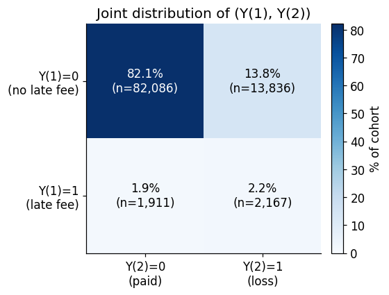
The mechanically-inherited contribution is real predictive content, it isn’t noise. I(Y^{(1)}; Y^{(2)}) may reflect shared latent risk factors, temporal structure, common causal mechanisms. The issue isn’t that this information is bad; it’s that knowing it is there doesn’t tell us whether the score itself has extracted any reusable feature-level structure. That’s the distinction the conditional measurement makes visible.
The diagnostic
The conditional mutual information
I\!\left(S^{(1)};\, Y^{(2)} \mid Y^{(1)}\right) \;=\; H\!\left(Y^{(2)} \mid Y^{(1)}\right) - H\!\left(Y^{(2)} \mid S^{(1)}, Y^{(1)}\right) \tag{1}
is the reduction in remaining uncertainty about the new target once the score is added to a conditioning set that already contains the original target. Practically, this isolates the score’s marginal contribution beyond the contribution already implied by target co-occurrence. Following the identity from the previous post, the conditional CMI is estimable as an out-of-sample log-loss gain: train one auxiliary model that uses only Y^{(1)} to predict Y^{(2)}, train another that uses (S^{(1)}, Y^{(1)}), subtract their per-example losses, average, cross-fit. The whole estimator is the expectation of the gap between two cross-entropies, one of which conditions on the score and one of which doesn’t. In practice, the quality of the auxiliary models matters substantially. Underfit auxiliaries underestimate the conditional information, while overfit auxiliaries can produce optimistic finite-sample estimates despite cross-fitting. The estimator should therefore be interpreted jointly with auxiliary-model diagnostics such as calibration and out-of-sample log-loss.
A concrete intuition helps here. Imagine two borrowers who both avoided late fees, so Y^{(1)} = 0 for both. One borrower received a late-fee-risk score of 0.49 and the other 0.01. Once we condition on the realised target Y^{(1)}, the binary event itself no longer distinguishes them, but the score still does. If the borrower with the higher score later charges off more often, then the score contains feature-level structure relevant to Y^{(2)} beyond the coarse binary realisation of Y^{(1)}. That residual differentiation is exactly what I(S^{(1)}; Y^{(2)} \mid Y^{(1)}) measures.
Three regimes are worth naming, keyed on the magnitude of I(S^{(1)}; Y^{(2)} \mid Y^{(1)}) relative to the score’s self-information I(S^{(1)}; Y^{(1)}):
- Near zero. The score adds nothing about Y^{(2)} beyond what Y^{(1)} already encodes, it is a target-specific score whose apparent cross-target performance is entirely accounted for by target co-occurrence.
- Comparable to the self-information. The score has extracted feature-dependent structure that survives the binary Y^{(1)} projection and remains predictive of Y^{(2)} on its own.
- In between. Partial portability, some feature-level structure carries over, some doesn’t.
These are heuristic practitioner interpretations rather than formally calibrated thresholds. Also, none of these readings is decisional on its own: a high CMI is necessary for the existing score to carry reusable predictive structure, but it is not sufficient to conclude that retraining is unnecessary. A fresh model trained on Y^{(2)} may still extract additional signal from X not captured by S^{(1)}.
The mechanism can be thought of as pure data-processing: S^{(1)} is a continuous summary of X, compressed through the lens of Y^{(1)}. Even after conditioning on whether Y^{(1)} = 1 actually occurred for an example, the score retains how likely it was that Y^{(1)} = 1 given X, and that continuous uncertainty often correlates with the features driving Y^{(2)} independently of Y^{(1)}’s realised value. In our lending example, a score trained to predict late-fee events carries the model’s continuous view of applicant riskiness; even after observing the binary late-fee outcome, the finer-grained risk estimate predicts terminal default beyond what the binary indicator does.
The interpretation is cleanest when S^{(1)} is approximately Bayes-optimal, i.e., when S^{(1)}(X) \approx P(Y^{(1)} = 1 \mid X). With a finite-capacity, miscalibrated, underfit, or overfit score, the diagnostic mixes target portability with the score’s representational quality. A low CMI may then mean “the targets are not portably linked through the features” or “this particular score didn’t extract enough of the structure that is there.” The cleanest framework run pairs the diagnostic with the retraining baseline introduced later in the post.
A word on the conditioning variable
A natural objection at this point: Y^{(1)} is also a future label. At deployment time, when we want to predict Y^{(2)}, we don’t observe Y^{(1)} either. Why is it permissible to condition on it?
The CMI is a retrospective structural diagnostic, not an operational predictor. We compute it on historical data, where both Y^{(1)} and Y^{(2)} have resolved. Y^{(1)} enters as a conditioning variable in a measurement, not as a feature of a deployable predictor. The score itself remains a function of X alone at deployment; the CMI is training-time bookkeeping that tells us what the score has encoded. Using Y^{(1)} as a feature of the deployed model would be temporal leakage. We aren’t doing that. Two different uses of Y^{(1)}, only one of which would be problematic.
What the CMI is not
A note on what one might be tempted to say but shouldn’t. It is not the case that the marginal MI decomposes additively into label-overlap plus score-specific contribution. The seductive-but-wrong identity is
I\!\left(S^{(1)}; Y^{(2)}\right) \overset{?}{=} I\!\left(Y^{(1)}; Y^{(2)}\right) + I\!\left(S^{(1)}; Y^{(2)} \mid Y^{(1)}\right). \tag{2}
That is not the chain rule. The actual chain rule decomposes the joint MI of the pair (S^{(1)}, Y^{(1)}) with Y^{(2)}:
I\!\left(S^{(1)}, Y^{(1)};\, Y^{(2)}\right) = I\!\left(Y^{(1)}; Y^{(2)}\right) + I\!\left(S^{(1)}; Y^{(2)} \mid Y^{(1)}\right).
Equating with the symmetric expansion gives the correct identity
I\!\left(S^{(1)}; Y^{(2)}\right) = I\!\left(Y^{(1)}; Y^{(2)}\right) + I\!\left(S^{(1)}; Y^{(2)} \mid Y^{(1)}\right) - I\!\left(Y^{(1)}; Y^{(2)} \mid S^{(1)}\right),
with a residual term that vanishes only under the strong assumption Y^{(1)} \perp Y^{(2)} \mid S^{(1)}, which fails generically. So the cross-target CMI is not “the score-specific share of marginal MI.” It is the score’s marginal contribution to predicting Y^{(2)} beyond Y^{(1)}, full stop. In the partial-information-decomposition sense (Williams & Beer, 2010), the quantity conflates unique-score content with synergistic content, a conflation it shares with the unique score contribution I(S^{(2)};Y^{(2)} \mid S^{(1)}), the ensemble decision diagnostic, the subject of the next post. This matters because the CMI tells us about the structure of what the score has encoded, not directly about the decision of whether to retrain. It’s a portability diagnostic.
Validating the estimator
Before pointing the estimator at real data, it’s worth confirming it recovers the truth in a setup where the truth is computable. The cleanest one is a bivariate-probit DGP where two correlated binary targets share a common predictor signal:
X \sim \mathcal{N}(\mathbf{0}, I_d), \quad g(X) = \beta_0 + X \beta, \quad (\nu_1, \nu_2) \sim \mathcal{N}\!\left(\mathbf{0}, \begin{pmatrix} 1 & \rho \\ \rho & 1 \end{pmatrix}\right)
with Y^{(j)} = \mathbb{1}[g(X) + \nu_j > 0] for j = 1, 2. The correlation \rho controls how aligned the two targets are. As \rho \to 1 the targets become identical and the cross-target CMI must collapse to zero; at \rho = 0 the targets are conditionally independent given X, but remain marginally dependent through the shared signal g(X) and the score’s continuous summary of that signal carries information about Y^{(2)} beyond what the coarse Y^{(1)} indicator captures. We plug in the population-optimal score S^{(1)}(X) = \Phi(g(X)) directly — the score-fitting step was already validated in the previous post and isn’t what this simulation is testing.
fig, ax = plt.subplots(figsize=(7, 3.6), constrained_layout=True)
ax.plot(rhos, truth, lw=2, label="truth", color="#3b82c4")
ax.errorbar(rhos, emp_mean, yerr=emp_se, fmt="o", capsize=3,
            color="#e88c30", label="cross-fitted estimate")
ax.set_xlabel(r"$\rho$  (target-noise correlation)")
ax.set_ylabel(r"$I(S^{(1)}; Y^{(2)} \mid Y^{(1)})$  (nats)")
ax.legend(frameon=False)
ax.grid(alpha=0.3)
plt.show()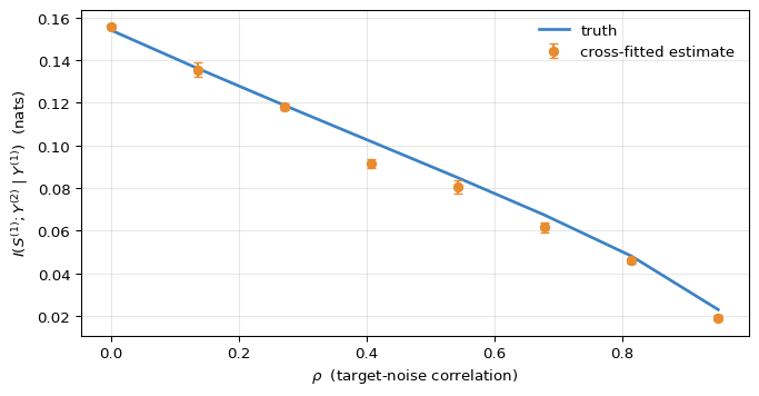
Figure 2 is the validation we want. The estimator’s behaviour across the sweep matches the closed-form truth: the qualitative shape is right, the collapse to zero at high \rho is captured, and the agreement is well within the cross-fit variability bars across most of the range. There is a small downward bias in the midrange that traces to the finite capacity of the GBDT auxiliary; richer auxiliaries or more samples reduce it but the qualitative reading is unchanged. With the estimator defended, we can point it at real data.
Real data: Lending Club
Lending Club’s loan-level dataset has rich application-time features and multiple resolvable outcomes per loan, which makes it natural ground for a cross-target portability question. The setup:
Cohort. Loans with a 36-month term and terminal status (Fully Paid, Charged Off, Default, plus the “Does not meet credit policy” variants of each). About 1.02M loans; we subsample to 100k for tractability.
Targets. Y^{(1)} is the indicator that the loan accrued at least one late-payment fee during its life (total_rec_late_fee > 0); Y^{(2)} is the indicator that it ended in loss (Charged Off or Default). Both are post-origination outcomes; both are observable retrospectively in the historical sample. Their joint distribution: P(Y^{(1)} = 1) \approx 4\%, P(Y^{(2)} = 1) \approx 16\%, the two off-diagonals of the 2×2 joint are both populated, and neither target contains the other.
Score. S^{(1)} is a histogram-GBDT trained out-of-fold (K=5 stratified folds) on (X, Y^{(1)}) with application-time features only — no payment-history fields, no post-origination FICO, nothing that could leak. The model’s job here is just to be a credible learned score; we aren’t testing the score-fitting machinery, only its cross-target behaviour.
The cross-target triad and the AUC comparison:
| on Y^{(1)} | on Y^{(2)} | |
|---|---|---|
| Base rate | 4.04% | 16.01% |
| AUC(S^{(1)}, \cdot) | 0.653 | 0.648 |
| \widehat I(S^{(1)}; \cdot) | 0.0054 \pm 0.0003 nats | 0.0188 \pm 0.0006 nats |
and the conditional quantity:
\widehat I\!\left(S^{(1)};\, Y^{(2)} \mid Y^{(1)}\right) \;=\; 0.0158 \pm 0.0005 \text{ nats}.
Two things are interesting in this table. First, the score is more informative about the cross-target than about its own training target, I(S^{(1)}; Y^{(2)}) > I(S^{(1)}; Y^{(1)}) in raw nats. That isn’t a mistake. One possible interpretation is that the features driving late-fee accrual overlap substantially with the features driving charge-off, and that the model trained on Y^{(1)} ends up extracting a representation more aligned with the broader credit-risk structure captured by Y^{(2)}. Another possibility is simply that the two targets differ in noise level, prevalence, or predictability in ways that make the cross-target information larger on this scale. The diagnostic itself does not distinguish among these mechanisms; it only tells us that the score carries substantial predictive content for Y^{(2)}.
Second, the conditional CMI’s magnitude is about 84% of the marginal CMI’s. That ratio is descriptive only: it should not be read as a chain-rule decomposition (as the next section makes explicit, the chain rule applies to the joint pair (S^{(1)}, Y^{(1)}), not to S^{(1)} alone). What it does indicate, qualitatively, is that the score’s predictive content for Y^{(2)} doesn’t shrink much when Y^{(1)} enters the conditioning. The score isn’t primarily relying on target co-occurrence; most of what it knows about Y^{(2)} is feature-level structure that survives projection through the binary Y^{(1)} outcome.
The retraining baseline
The conditional CMI alone can’t tell us whether 0.0158 nats is “most of what’s achievable” or “a small fraction of it.” That needs a baseline. Train a same-architecture, same-features model directly on Y^{(2)}, call it S^{(2)}, and compute its conditional CMI:
\widehat I\!\left(S^{(2)};\, Y^{(2)} \mid Y^{(1)}\right) \;=\; 0.0284 \pm 0.0007 \text{ nats},
with \widehat{\text{AUC}}(S^{(2)}, Y^{(2)}) = 0.692. The retrained model extracts almost twice the conditional information from the same features. The portability ratio — the fraction of the retraining baseline that the cross-target score captures —
\frac{\widehat I(S^{(1)};\, Y^{(2)} \mid Y^{(1)})}{\widehat I(S^{(2)};\, Y^{(2)} \mid Y^{(1)})} \;\approx\; 56\%
is the practitioner-relevant scalar. This suggests the score has partial portability, not full.
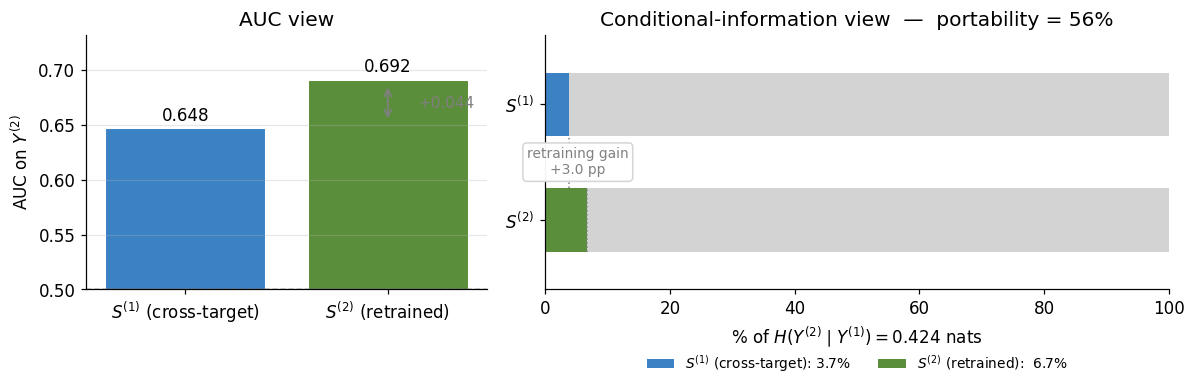
The AUC and CMI views agree in direction: both say retraining helps. They disagree in magnitude. AUC reads as a small improvement; the normalised CMI reads as nearly doubling the information extracted. Both are correct statements about the same data. Reporting only one risks miscalibration — AUC alone would understate the retraining gap; CMI alone would lack the familiar discrimination scale practitioners use to ship models.
To stress-test the stability of this picture, the same pipeline run with two additional random seeds gives portability ratios of 55.2% and 51.5% respectively — within fold-level standard errors of the seed-0 result. The qualitative conclusion is not riding on a lucky split.
What this doesn’t tell you
The cross-target CMI answers a structural question about the score and informs the retraining decision, but it doesn’t make the decision. Four caveats worth naming explicitly:
The information-theoretic quantity that most directly addresses “should I retrain?” is not this conditional CMI. It is the unique score contribution, I(S^{(2)}; Y^{(2)} \mid S^{(1)}) — given the existing score, does the retrained model add anything orthogonal? That’s the headline of the next post in this series. The cross-target CMI is the cheap diagnostic computed before training the alternative; the unique-score-contribution CMI is the diagnostic computed after.
The cross-target CMI conflates unique-score content with synergistic content in the partial-information-decomposition sense. It measures the score’s marginal contribution beyond Y^{(1)}, including any synergy that emerges from observing (S^{(1)}, Y^{(1)}) jointly. For most product decisions this conflation is benign, but it is worth knowing.
The features in the Lending Club analysis include int_rate, grade, and sub_grade, which encode LC’s own internal risk model. A score trained on these features partly imitates LC’s grading model rather than learning the underlying credit-risk structure from scratch. The portability claim inherits whatever LC’s grading model encodes. A cleaner experiment would drop these features and rerun; the qualitative conclusion is unlikely to flip but the absolute numbers would shift.
The log-loss-gain estimator is calibration-sensitive. HistGBDT outputs aren’t strongly calibrated by default. A natural robustness check is to refit the full auxiliary as an isotonic regression stratified by Y^{(1)} and verify the estimate doesn’t move. The seed-stability check above is some evidence that calibration isn’t doing the heavy lifting, but it isn’t a substitute for a direct calibration audit.
Real-world retraining decisions also include deployment friction, audit requirements, downstream consumers of the existing score — operational inputs that don’t appear in any CMI. The diagnostic informs the decision; it doesn’t replace the operational judgment that surrounds it.
In one paragraph
The conditional mutual information framework provides a principled way to distinguish mechanically-inherited target overlap from genuinely portable predictive structure. Rather than asking whether a score appears predictive for a second target in aggregate — which AUC and marginal MI both do, and which conflates the two contributions — I(S^{(1)}; Y^{(2)} \mid Y^{(1)}) asks whether the score still differentiates outcomes once the original target realisation is held fixed. A positive value indicates that the score has extracted feature-dependent structure relevant to the new target beyond simple label co-occurrence. Crucially, this does not prove that retraining is unnecessary; it quantifies how much reusable structure the existing score already contains, providing a rigorous diagnostic for deciding whether retraining is likely to be valuable. Two decision-relevant quantities sit one chain rule downstream — the replacement diagnostic I(S^{(2)}; Y^{(2)} \mid S^{(1)}) (does retraining add information the existing score doesn’t already carry?) and the ensemble diagnostic I(S^{(1)}; Y^{(2)} \mid S^{(2)}) (does the existing score still contribute anything when stacked with a retrained one?) — and are the subject of the next post.
What’s next
The next post stays inside the same chain-rule decomposition but moves the conditioning set from a label to a score. Both sides of the chain rule become decision-relevant: the ensemble diagnostic I(S^{(1)}; Y^{(2)} \mid S^{(2)}) asks whether the existing score still contributes anything once stacked with the retrained one; the replacement diagnostic I(S^{(2)}; Y^{(2)} \mid S^{(1)}) asks whether the retrained score carries information the existing one doesn’t. Same cross-fitting machinery, same log-loss gain identity, same PID conflation caveats — different conditioning set, different practitioner decisions. The framework’s coherence comes from the fact that self-information, cross-target CMI, and the two score-conditioned diagnostics are all the same calculation with different choices of Z.
One-liner
The cross-target CMI measures how much of a score’s predictive content for a new target survives projection through the original target. It is a portability diagnostic, not a retraining decision rule — its decision-relevant siblings (the ensemble and replacement diagnostics) sit one chain rule downstream and are the subject of the next post.
References
Williams, P. L., & Beer, R. D. (2010). Nonnegative decomposition of multivariate information. arXiv Preprint arXiv:1004.2515. https://arxiv.org/abs/1004.2515