Should I retrain my score, ensemble it, or both?
You already have a score in production and you’ve retrained it. Should you replace the old one, or keep both and build an ensemble? At first glance those sound like the same question. They are not. On Lending Club, they give opposite answers.
The previous post ended with a number and a promise. The number was the portability ratio. The promise was that we would stop asking how portable is this score? and ask the question practitioners actually care about: should I retrain it?
It turns out that this is the wrong question.
Or rather, it bundles together two different decisions. Suppose you already have a score running in production and you retrain it on a better target. Should you replace the old score? Or should you keep both and build an ensemble? At first glance those sound like different ways of asking the same thing. They are not. One asks whether the new score contains information the old one is missing. The other asks whether the old score still has anything left to contribute once the new one is available.
The nice surprise is that information theory separates these two questions almost for free. Both answers come from the same chain rule, both are computed with exactly the same estimator, and both differ only in which score appears in the conditioning set.
Two questions, one decomposition
Before any math, an intuition. Picture two Lending Club borrowers. Both get the same cross-target score, S^{(1)} = 0.32. The retrained score handles them differently. One gets S^{(2)} = 0.21, the other S^{(2)} = 0.45. If that gap continues to predict charge-off on held-out folds, then S^{(2)} knows something about Y^{(2)} that S^{(1)} does not. The replacement diagnostic is the population-level version of that observation. It is the answer to the question: what does S^{(2)} tell us about Y^{(2)} once S^{(1)} is already held fixed?
Now the math. The chain rule for mutual information (Wyner, 1978) decomposes the joint MI of two scores with a target in two equivalent ways:
\begin{aligned} I\!\left(S^{(1)}, S^{(2)}; Y^{(2)}\right) &= I\!\left(S^{(2)}; Y^{(2)}\right) + \underbrace{I\!\left(S^{(1)}; Y^{(2)} \mid S^{(2)}\right)}_{\text{ensemble diagnostic}} \\ &= I\!\left(S^{(1)}; Y^{(2)}\right) + \underbrace{I\!\left(S^{(2)}; Y^{(2)} \mid S^{(1)}\right)}_{\text{replacement diagnostic}}. \end{aligned} \tag{1}
The same population quantity, split two ways. Each split corresponds to a different practitioner question.
The ensemble diagnostic I(S^{(1)}; Y^{(2)} \mid S^{(2)}) asks: if we already have the retrained score S^{(2)} deployed, what does adding the cross-target score S^{(1)} buy us? From the equivalence in post 1, the quantity equals the exact expected per-example log-loss reduction we would see by stacking S^{(1)} on top of S^{(2)} in a calibrated meta-model.
The replacement diagnostic I(S^{(2)}; Y^{(2)} \mid S^{(1)}) asks the inverse. If we have S^{(1)} in production today, what does the retrained score add beyond it? The quantity equals the expected log-loss reduction conditional on having S^{(1)} available. It is not quite the standalone gain we would see if we used S^{(2)} alone after dropping S^{(1)}. It bounds that gain from above. We come back to the asymmetry a few sections down.
We deliberately name them after the decision each informs. The label tracks the practitioner question, not the score appearing on the left side of the conditional. Both are valid splits of the same joint MI. Both are equally well-defined as population quantities. They simply answer different questions.
What changes when the conditioning set is a score
The only change from the previous post sounds small. Instead of conditioning on a binary label, we condition on another score. Operationally that is a tiny shift. But it changes the estimation problem in an important way.
In post 2 the conditioning variable was Y^{(1)}, a binary label. The baseline auxiliary \hat{p}_0(Y^{(2)} \mid Y^{(1)}) was a two-cell lookup. We counted how often Y^{(2)} = 1 for examples with Y^{(1)} = 0, and how often for Y^{(1)} = 1. Two numbers, both essentially noiseless. The only model that carried estimation noise was the full auxiliary \hat{p}_1(Y^{(2)} \mid S^{(1)}, Y^{(1)}).
When the conditioning variable is a score, the baseline stops being a table. \hat{p}_0(Y^{(2)} \mid S^{(2)}) becomes a regression on a continuous covariate. In our implementation it is a 1D HistGBDT. The full auxiliary \hat{p}_1(Y^{(2)} \mid S^{(1)}, S^{(2)}) is a 2D HistGBDT. Both legs of the log-loss difference now carry estimation noise.
Three practical consequences follow.
First, the finite-sample bias of the estimator becomes more visible. In the label-conditional setting, the baseline’s variance contribution was dwarfed by the full auxiliary’s. With two flexible auxiliaries differenced, finite-sample bias of both contributes. Honest reporting includes a fold-level standard error and a seed-variation check.
Second, out-of-fold score generation is no longer optional. If we naively train S^{(2)} on all the data and then condition on it when predicting Y^{(2)}, we leak Y^{(2)} into the conditioning set, and the quantity we end up estimating is not the one we wanted. The score being conditioned on has to itself be an out-of-fold prediction on the rows where the CMI is evaluated. The pipeline from post 2 already does this for both S^{(1)} and S^{(2)}.
Third, the population quantity is well-defined for arbitrary continuous conditioning. The measure-theoretic foundation (Wyner, 1978) earns its keep here. I(S; Y \mid Z) is defined via a supremum over finite-partition approximations and requires no regularity assumptions on Z’s distribution. Continuous scores from trained models are exactly the case the construction was built for.
The estimator itself is a small extension of the cross-fitting harness from posts 1 and 2:
def cf_score_conditional_cmi(S_a, S_b, Y, K=5, seed=0):
    """Cross-fitted Î(S_a; Y | S_b) via the log-loss-gain identity."""
    fold_means = []
    for tr, te in StratifiedKFold(K, ..., random_state=seed).split(S_a, Y):
        # 1D HistGBDT on S_b -> Y          (baseline auxiliary)
        m0 = HistGradientBoostingClassifier(...).fit(S_b[tr, None], Y[tr])
        p0 = m0.predict_proba(S_b[te, None])[:, 1]
        # 2D HistGBDT on (S_a, S_b) -> Y   (full auxiliary)
        m1 = HistGradientBoostingClassifier(...).fit(
            np.column_stack([S_a[tr], S_b[tr]]), Y[tr])
        p1 = m1.predict_proba(np.column_stack([S_a[te], S_b[te]]))[:, 1]
        fold_means.append((loss(Y[te], p0) - loss(Y[te], p1)).mean())
    return np.mean(fold_means), np.std(fold_means, ddof=1)/np.sqrt(K)
To switch from the ensemble diagnostic to the replacement diagnostic, we swap the order of S_a and S_b. The code is identical for the two quantities. Only the practitioner question is different.
What the number measures, and what it doesn’t
At the level of log-loss, both quantities have a clean operational meaning. The ensemble diagnostic equals the expected per-example log-loss improvement we would see by replacing a predictor that uses only S^{(2)} with one that uses both scores jointly. The replacement diagnostic equals the analogous improvement when we replace a predictor that uses only S^{(1)} with one that uses both. Both identities follow from the chain rule and the log-loss-gain identity from post 1.
What is less clean is the match between each quantity and the practitioner decision it is meant to inform.
For the ensemble decision, the math and the question line up. We are deploying both scores. If the pair (S^{(1)}, S^{(2)}) carries information about Y^{(2)} that neither marginal carries on its own, that interaction structure is available to us exactly when we observe both scores. The ensemble quantity measures that signal, and the ensemble decision is in a position to use it.
For the replacement decision, the alignment breaks. We are dropping S^{(1)} and using S^{(2)} alone. Any signal that requires observing both scores jointly disappears the moment we stop seeing S^{(1)}. The replacement quantity still counts that signal in its CMI value, though. What we get from it is an upper bound on the part of S^{(2)}’s contribution that survives dropping S^{(1)}. Equivalently, it is an upper bound on the standalone log-loss gain from switching.
Partial-information decomposition (Williams & Beer, 2010) begins exactly here. In that framework, the joint MI splits into four non-negative parts: I(S^{(1)}, S^{(2)}; Y^{(2)}) = \text{Unq}_1 + \text{Unq}_2 + \text{Red} + \text{Syn}, with the consistency identity I(S^{(j)}; Y^{(2)} \mid S^{(k)}) = \text{Unq}_j + \text{Syn}. Both of our diagnostics carry \text{Unq} + \text{Syn}. What differs is whether the decision they inform tolerates the \text{Syn} part. We do not pick a redundancy measure here. That is the subject of the next post. The distinction matters for honest reporting now.
One terminological note. The two diagnostics are not symmetric. They measure different things and inform different decisions. Naming them only by the variable on the left-hand side would obscure the decision each is meant to inform.
Validating the estimator
Before the LC numbers, a controlled DGP where the truth is computable. We want the validation to make the marginal-vs-conditional divergence visible and analytically tractable, without smuggling in a PID commitment we’d rather defer.
We start with two independent binary latents U, V \sim \text{Bernoulli}(1/2) and build continuous scores S^{(1)} = U + \eta_1, S^{(2)} = V + \eta_2 with small Gaussian noise \eta_j \sim \mathcal{N}(0, \sigma^2). The target follows a one-parameter mixture:
P(Y = 1 \mid U, V) = (1 - \alpha) \cdot \frac{U + V}{2} \;+\; \alpha \cdot (U \oplus V), \tag{2}
where the knob \alpha \in [0, 1] interpolates from an additive-risk endpoint (the conditional probability is additive in U and V) to a pure-XOR endpoint (the conditional is XOR-shaped). At the additive endpoint the marginal MIs I(U; Y) and I(V; Y) are both positive; at the XOR endpoint they vanish exactly, and all predictive content lives in the joint (U, V). The marginal label rate is held at P(Y = 1) = 1/2 for every \alpha — the dial moves only the structure of P(Y \mid U, V), not the unconditional rate. The dial controls interaction structure, not the synergy term of any PID decomposition; PID claims at either endpoint would require committing to a redundancy measure, which the validation deliberately doesn’t.
Because the joint distribution at the latent level is fully analytic, the corresponding population MIs — I(V; Y), I(V; Y \mid U), I(U, V; Y) — can be computed by direct enumeration over the four (U, V) configurations. They serve as reference curves for the empirical estimator applied to the noisy continuous scores.
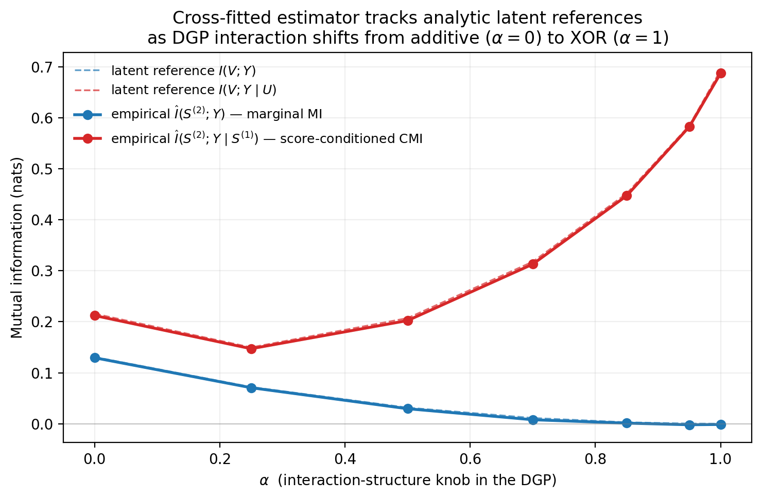
Notice what happens between the two solid lines as \alpha grows. At the additive endpoint the marginal MI and the conditional CMI sit within a factor of about 1.7 of each other. The conditional CMI is roughly what a calibrated standalone evaluation of S^{(2)} would tell us. At the XOR endpoint, the marginal MI collapses to zero. Neither score individually predicts Y. But the conditional CMI reaches the full joint information, \ln 2 \approx 0.693 nats. A reader looking only at marginal MIs would conclude the scores are useless. The conditional says they are each fully informative once the other one is observed. The structural mismatch between marginal and conditional MI is exactly what the score-conditioned estimator is built to detect.
The empirical curves track their latent references to within 0.006 nats at every \alpha, with a mean absolute deviation of 0.002 to 0.004 nats. The cross-fitted estimator is faithfully recovering the underlying information-theoretic trends. The next section asks whether the same mismatch shows up on Lending Club.
Lending Club: ensemble vs replacement on real data
The cohort is the same one from post 2: 200,000 36-month-term loans with terminal status. Y^{(1)} is “loan accrued at least one late fee” (p = 4.0\%); Y^{(2)} is “loan ended in loss — charged off or defaulted” (p = 16.0\%). Both scores are fit with the same architecture (HistGBDT, max_iter = 400, depth 6) on application-time features, generated out-of-fold across K = 5 stratified folds. The standalone discrimination metrics tell the familiar story:
| metric | S^{(1)} (cross-target) | S^{(2)} (retrained) |
|---|---|---|
| AUC vs Y^{(2)} | 0.6526 | 0.6953 |
| \widehat{I}(\cdot; Y^{(2)}), nats | 0.0204 ± 0.0001 | 0.0327 ± 0.0002 |
The retrained model has about five AUC points and about 60% more marginal MI on its own target. So far, nothing surprising. Directly training on the target you care about beats borrowing a score trained on a related one.
Now the two new quantities. Both come from one call to cf_score_conditional_cmi. Only the order of the score arguments differs.
Ensemble diagnostic. Does the cross-target score add anything when stacked on top of the retrained one?
\widehat{I}\!\left(S^{(1)}; Y^{(2)} \mid S^{(2)}\right) \approx 0 \text{ nats}.
Statistically indistinguishable from zero (the raw cross-fitted estimate is -0.0002 \pm 0.0000). The slight negative sign reflects nuisance-model error near the boundary, not negative information. The population quantity is non-negative by Wyner’s Lemma 3.1 (Wyner, 1978). In practical terms, stacking S^{(1)} on top of S^{(2)} would deliver no measurable log-loss improvement. The retrained score subsumes whatever feature-level signal the cross-target score had picked up.
Replacement diagnostic. Does the retrained score carry information the cross-target one doesn’t?
\widehat{I}\!\left(S^{(2)}; Y^{(2)} \mid S^{(1)}\right) = +0.0124 \pm 0.0001 \text{ nats } \;(2.8\% \text{ of } H(Y^{(2)})).
Positive and well-determined. The retrained model carries about 0.012 nats of information about Y^{(2)} beyond what the cross-target score already encodes. That is roughly 38% of the retrained model’s standalone marginal MI.
What jumps out is the asymmetry. The two scores are not informationally symmetric on Y^{(2)}. S^{(2)} appears to contain essentially all of the charge-off-relevant information carried by S^{(1)}, plus a bit more. S^{(1)} contributes little beyond S^{(2)}. In information-theoretic terms, S^{(1)} appears to contain little Y^{(2)}-relevant information beyond what is already captured by S^{(2)}. In practical terms, if the retrained score is in production we do not need the cross-target one. If only the cross-target score is in production, retraining buys us a real but modest gain.
Connection to post 2’s 56% portability ratio. Post 2 computed \widehat{I}(S^{(1)}; Y^{(2)} \mid Y^{(1)}) / \widehat{I}(S^{(2)}; Y^{(2)} \mid Y^{(1)}) and got about 0.56. That ratio is the fraction of conditional information the cross-target score captures relative to direct retraining, with the binary Y^{(1)} in the conditioning set. The replacement diagnostic here measures something different. It is the additional information S^{(2)} provides beyond S^{(1)}, with no Y^{(1)} in the conditioning. Both are honest signals of what the cross-target score is missing relative to the retrained one. The post-2 framing was “how much of a same-architecture retrain is the cross-target score already delivering?”. The post-3 framing is “how much does the retrained score uniquely add on top of the existing one?”. The numbers come at the same underlying relationship from different directions, and they agree on the qualitative story. S^{(1)} has some real portable structure for Y^{(2)}. S^{(2)} has more. The additional content is small but well-determined.
Seed stability. Across all three loop seeds the per-seed estimates are essentially identical. Each diagnostic’s across-seed SE is at most 0.0002 nats. The qualitative conclusion is not riding on a lucky split. A methodological note. The across-seed SE here reflects K-fold split and nuisance-model RNG variation on a fixed subsample of the LC cohort. The subsample is drawn once and reused for every seed in the loop. It does not include data-sampling variability across different cohort subsamples. To probe that, we would rerun under different subsamples and compare.
What this doesn’t tell you
Four caveats, in order of importance:
The replacement diagnostic is an upper bound on the standalone gain from dropping S^{(1)} and using S^{(2)} alone. As discussed earlier, the conditional CMI counts unique-to-S^{(2)} content plus any synergistic signal that requires observing both scores jointly. If a substantial fraction of the diagnostic is synergistic, you would lose that signal when dropping S^{(1)}, and the actual switch-gain would be smaller than 0.012 nats. The partial-information decomposition needed to quantify this is the subject of the next post.
The features include int_rate, grade, and sub_grade — Lending Club’s own underwriting outputs. Both S^{(1)} and S^{(2)} inherit LC’s policy model. A cleaner experiment would drop these features and rerun; the qualitative ensemble/replacement asymmetry is unlikely to flip, but the magnitudes would shift.
Both auxiliary models in the score-conditioned estimator are HistGBDTs, calibrated only by training, not by post-processing. A natural robustness check is to refit the full auxiliary with isotonic regression on top and confirm the diagnostic doesn’t move. The synthetic validation suggests calibration sensitivity is small (the empirical curves track the latent references uniformly to within ~0.006 nats), but that’s evidence for the synthetic distribution, not for LC.
The across-seed SE doesn’t include data-sampling variability. The cohort is subsampled once with a fixed seed and reused for every fold seed. To probe data-sampling variability we would rerun the pipeline under different cohort subsamples. The seed-stability evidence above shows that fold + model RNG isn’t doing the heavy lifting, which is a necessary but not sufficient check.
Real retraining and deployment decisions also depend on operational inputs (model registry, monitoring, downstream consumers, audit requirements) that do not appear in any CMI. The diagnostics inform the decision. They do not replace the operational judgment around it.
In one paragraph
The chain-rule decomposition of I(S^{(1)}, S^{(2)}; Y^{(2)}) yields two conditional-CMI quantities, the ensemble diagnostic and the replacement diagnostic, that share one estimator but inform different practitioner decisions. The ensemble diagnostic is operationally exact for “should I stack S^{(1)} on top of S^{(2)}?”. The replacement diagnostic is an upper bound on “should I drop S^{(1)} and switch to S^{(2)}?”. The estimator extends post 2’s cross-fitting machinery, now with both auxiliaries flexible because the conditioning variable is a continuous score, and is validated against analytically computable latent-level references on a controlled synthetic DGP. On Lending Club, the ensemble diagnostic is statistically indistinguishable from zero, while the replacement diagnostic is positive and well-determined. The retrained score subsumes the cross-target one on charge-off: ensembling buys nothing, while switching buys about 0.012 nats, or 2.8% of the target’s total entropy. The clean asymmetry is consistent with the 56% portability ratio of post 2, and sharpens it.
What’s next
The replacement-diagnostic upper-bound caveat is the entry point for the next post. The next step is to separate two ideas that conditional MI keeps bundled together: information that belongs uniquely to one score, and information that only appears when both scores are read jointly. Partial-information decomposition (Williams & Beer, 2010) does exactly that. It splits the joint MI I(S^{(1)}, S^{(2)}; Y) into four non-negative parts: a unique-to-S^{(1)} piece, a unique-to-S^{(2)} piece, a redundant piece shared between them, and a synergistic piece that only emerges when both scores are observed together. The consistency identity I(S^{(j)}; Y \mid S^{(k)}) = \text{Unq}_j + \text{Syn} then makes precise the upper-bound caveat we have been carrying. The conditional CMI captures unique plus synergistic content. The next post picks a redundancy measure (likely BROJA, the most principled axiomatic candidate for binary targets) and walks through what the LC numbers say in PID coordinates. A natural hypothesis is that if the LC scores are mostly informationally redundant (which the ensemble-diagnostic-near-zero suggests), the synergy term will be small and the replacement diagnostic will be close to the true unique contribution of S^{(2)}. The upper-bound caveat would then be loose enough that “switching buys 0.012 nats” is approximately the unconditional truth, not just an upper bound.
One chain rule, two diagnostics. On Lending Club, the retrained score subsumes the cross-target one informationally. Ensembling buys nothing. Switching buys a small but well-determined gain.